Blogs

Bayesian Statistics Implementation

Anurag Gulati

03 Mar 2024 • 9 min read

How do we implement a typical Bayesian Inference?

Welcome to the blog where we dive into the world of Bayesian inference models! In this exploration, we'll unravel the magic of Bayesian statistics by implementing it in two practical examples. Get ready to demystify the Bayesian approach as we walk through real-world applications, sampling posterior distributions, and deriving insights from the interplay between prior beliefs and observed data.

Its really not important to understand each aspect of the code, however, it would be great to understand the ideology behind this entire exercise. So, please do not worry if you cannot get each aspect of the picture. Focus on the larger picture.

Problem 1

You're playing a coin-flipping game. After tossing the coin 100 times, it landed on heads 61 times. We call getting heads a "success." Now, the goal is to use a cool Bayesian method to figure out the chance of getting heads in future coin flips based on the data we just saw (the number of heads).

Solution:

Programming language - I have used Python programming language for the coding.

Explanation of the above code and understanding the concept (optional to understand)

1.) Number of Trials (n) and Observed Number of Heads (k):

• n = 100: This represents the number of trials or coin flips.k = 61: This is the observed number of "successes" (heads) in those trials.

• These are the details of the experiment which we performed to obtain the posterior probability

2.) PyMC3 Model Setup:

• with pm.Model() as coin_context:: This line initializes a PyMC3 model context. All subsequent model components will be defined within this context.

3.) Prior Distribution for Probability of Heads (p):

• p = pm.Uniform('p', 0.4, 0.8): This line specifies a prior distribution for the probability of getting heads (p) using a uniform distribution between 0.4 and 0.8. This reflects the belief or uncertainty about the probability of heads before observing any data. Note: This prior belief is irrespective of our experiment. We are assuming a uniform distribution of probability before we perform our experiment.

4.) Likelihood (Observation Model):

• y = pm.Binomial('y', n=n, p=p, observed=k): This line defines the likelihood or observation model. It assumes a binomial distribution for the observed data (y) given the parameters n (number of trials) and p (probability of success, i.e., getting heads). The observed parameter is set to the actual number of heads observed (k).

5.) Sampling from the Posterior:

• trace = pm.sample(1000): This line performs Bayesian inference by drawing 1000 samples from the posterior distribution using a sampling method (usually MCMC). The resulting samples are stored in the trace variable and will be used to make inferences about the posterior distribution of the parameters.

Forget about the code, just get the larger picture - Through below steps, it will be super clear to you.

Initial Beliefs: Start with what you initially think is the chance of success (heads in a coin flip), somewhere between 0.4 and 0.8. This is just your belief and has nothing to do with the experiment. This is "prior".
Flip the Coin 100 Times: Conduct an experiment by flipping the coin 100 times to gather real-world data.
Bayesian Model Comes In: Use a Bayesian model to update your beliefs based on the new data.
Posterior Probability Distribution: The model provides a "posterior probability distribution," refining your initial beliefs by considering uncertainties in the data.
Understanding the Distribution: This distribution illustrates the range of potential success probabilities, accounting for the uncertainty in the observed data.
Random Sampling: Randomly select 1000 values from this distribution to represent different potential success rates.
Review the Results: Examine the 1000 values to understand the spectrum of success probabilities based on the updated model, incorporating insights from the coin flips.

Finally, from the updated beliefs (posterior distribution), you randomly sample 1000 values of probability and generate below output.

From the same 1000 samples, you can extract mean or median or standard deviation to deduce point estimates, which is all you would do using frequentist approach. See below.

The mean from the 1000 samples is 0.61, which is close to what we observed from the experiment (performed 100 times).

Problem 2

We're looking at Gapminder data, a collection of country-level information over time. For our study, we'll zoom in on two things: proportion of babies under 5 surviving and the number of babies per woman in different countries. Our hypothesis is that one of these factors influences the other. Using Bayesian modeling, we're going to figure out how much they're connected. It might sound like a regression problem, and indeed it is! In this case, we're going to use Bayesian modeling to estimate the key numbers (coefficient and intercept) in our regression model.

Solution

Lets first look at the glimpse of the data and the two metrics we are talking about.

Note that I have filtered for the latest year in the data, i.e., 2015. We will focus on the rest of the analysis as per 2015 to remove bias of any kind and for simplistic purpose.

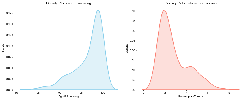
Next, lets look at the distribution of the two metrics in consideration side by side.

Distribution of the two metrics - age_5_surviving & babies per woman

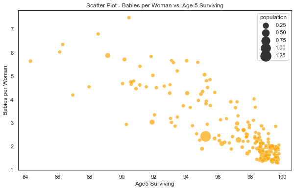
Now, lets look at the scatter plot of the two metrics as per 2015 statistics. Note that each bubble in below chart represents a country.

Its super clear that there is an inverse relationship between the two metrics. The countries with high proportion of babies surviving have lower babies per woman. Bingo! We just need to quantify this relationship using Bayesian modelling. So, lets go ahead then.

💡

Firstly, let's clarify our goal with this modeling effort. We're aiming to understand and obtain the distribution of two key elements: the slope and intercept. Why? Well, in a linear regression model, these two parameters are crucial. Instead of just pinpointing specific values for them, we're going the Bayesian modeling route to reveal their entire distributions. Once we have these distributions, we can then extract point estimates, providing us what we would exactly want.

See the python code below (optional):

Code for regression modelling using Bayesian approach

Further explanation of above code is given in a fundamental way below. Feel free to skip.

Explanation of the above code and understanding the concept (optional to understand)

PyMC3 Model Setup:
- with pm.Model() as gapminder_context:: This line initializes a PyMC3 model context named gapminder_context. All subsequent model components will be defined within this context.
Model Parameters:
- intercept = pm.Uniform('intercept', 5, 15): This line defines a uniform prior distribution for the intercept parameter. The intercept represents the value of the dependent variable when all independent variables are zero. The prior is uniform between 5 and 15. This is just our assumption (hence prior belief).
- slope = pm.Uniform('slope', -1, 1): This line defines a uniform prior distribution for the slope parameter. The slope represents the change in the dependent variable for a one-unit change in the independent variable. The prior is uniform between -1 and 1. This is just our assumption (hence prior belief).
Likelihood (Observation Model):
- babies = pm.Normal('babies', mu=intercept + slope * (gdata_2015['age5_surviving'] - 65), sd=1, observed=gdata['babies_per_woman']): This line defines the likelihood or observation model. It assumes a normal distribution for the observed data (gdata['babies_per_woman']) with a mean (mu) given by the linear regression model. The linear regression model is defined as intercept + slope * (gdata_2015['age5_surviving'] - 65). The standard deviation (sd) is set to 1.
Sampling from the Posterior:
- trace = pm.sample(1000): This line performs Bayesian inference by drawing 1000 samples from the posterior distribution using a sampling method (usually MCMC). The resulting samples are stored in the trace variable and will be used to make inferences about the posterior distribution of the parameters.

Simple explanation:

Model Purpose: The code establishes a Bayesian linear regression model to explore how the number of babies per woman relates to the survival rate of babies aged 5 and below.
Parameter Priors: It assigns uniform priors to the intercept and slope parameters. These priors represent our initial beliefs about these parameters.
Likelihood Modeling: The likelihood of our model is shaped as a normal distribution. The mean of this distribution follows the linear regression equation.
Posterior Distribution Sampling: The code then samples the posterior distribution of the parameters. This gives us a range of parameter values that align with both our initial beliefs (priors) and the data we've observed.
Resulting Insights: Ultimately, this process provides us with a set of parameter values that are in harmony with our prior beliefs and the actual data we have.

In summary, this code sets up a Bayesian linear regression model for the relationship between the number of babies per woman and the age-5 survival rate. The intercept and slope parameters are assigned uniform priors, and the likelihood is modeled as a normal distribution with mean given by the linear regression equation. The posterior distribution of the parameters is then sampled to obtain a set of parameter values that are consistent with both the prior beliefs and the observed data.

Lets look at the outputs of this exercise.

The mean from the 1000 samples is 13.8 for intercept and -0.35 for slope, which is what we achieved as point estimates using this model. Got it? This is what a researcher would use in the end, so even if you understood the gist, its okay too.

Since we said that we are generating the distribution of slope and intercept, lets just look at those distributions.

Distribution of slope and intercept for the 1000 samples we collected

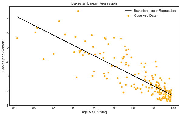
Finally, lets plot the regression line between the two metrics using the point estimates (averages of the 1000 sampled values from the posterior distribution).

Summary

We implemented Bayesian inference modelling for two problems. Any problem can be solved through a similar approach. Below are the steps that need to be followed for implementing a Bayesian model.

Navigation of prior probability
Designing likelihood function
Designing the Bayesian model
Sensitivity analysis (by choosing different prior/initial beliefs & likelihood criteria)

Again, not mandatory to learn everything. In the end, if you remember the following:

Initial Beliefs + New Evidence = Posterior Beliefs

This should also be enough for understanding the overall concept😄

Explanation of the above code and understanding the concept (optional to understand)

Explanation of the above code and understanding the concept (optional to understand)

Summary

References: